The ungriddedTableDef element
defines a set of non-orthogonal data points, along with their independent values
(coordinates), corresponding with the dependent value of an arbitrary function.
A 'non-orthogonal' data set, as opposed to a gridded or 'orthogonal' data set, means that the independent values are not laid out in an orthogonal grid. This form must be used if the dependent coordinates in any table dimension cannot be expressed by a single monotonically increasing vector.
See the excerpts below for two instances of ungridded data.
An optional
uncertainty
element may be provided that represents the statistical variation in the values
presented. See the section on Statistics below for more
information about this element.
    ungriddedTableDef : utID, [name, units]
        description? :
            {description character data}
        EITHER
            provenanceRef? : provID
        OR
            provenance? : [provID]
                author+ : name, org, [email]
                    contactInfo* : [contactInfoType, contactLocation]
                        {text describing contact information}
                creationDate : date {in YYYY-MM-DD format}
                documentRef* : [docID,] refID
                modificationRef* : modID
                description?
        uncertainty? : effect
            (normalPDF : numSigmas) | (uniformPDF : bounds+)
        dataPoint+ :
            {coordinate/value sets as character data}
ungriddedTableDef
attributes:
ungriddedTableDef
sub-elements:
-
description The optional description element allows the author to describe the data contained within this
ungriddedTable.-
provenance The optional provenance element allows the author to describe the source and history of the data within this
ungriddedTable. Alternatively, aprovenanceRefreference can be made to a previously defined provenance.-
uncertainty This optional element, if present, describes the uncertainty of this parameter. See the section on Statistics below for more information about this element.
-
dataPoint One or more sets of coordinate and output numeric values of the function at various locations within its input space. This element includes one coordinate for each function input variable. Parsing this information into a usable interpolative function is up to the implementer. By convention, the coordinates are listed in the same order that they appear in the parent function.
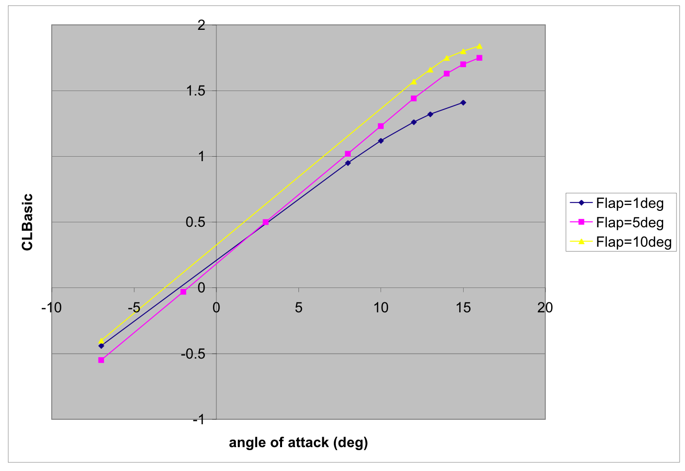
Example 9.
An excerpt showing an ungriddedTableDef element, encoding the data
depicted in Figure 2.
This 2D function table is an example provided by Dr. Peter
Grant of the University of Toronto. Such a table definition would be used in a
subsequent function to describe how an output variable would be
defined based on two independent input variables. The function table does not indicate
which input and output variables are represented; this information is supplied by the
function element later so that a single function table can be reused
by multiple functions.
<ungriddedTableDef name="CLBASIC as function of flap angle and angle-of-
attack" utID="CLBAlfaFlap_Table" units="nd">
<description>
CL basic as a function of flap angle and angle-of-attack. Note the alpha
used in this table is with respect to the wing design plane (in degrees).
Flap is in degrees as well.
</description>
<provenance>
<author name="Peter Grant" org="UTIAS"/>  <creationDate date="2006-11-01"/>
<documentRef refID="PRG1" />
</provenance>
<!--For ungridded tables you provide a list of dataPoints-->
<creationDate date="2006-11-01"/>
<documentRef refID="PRG1" />
</provenance>
<!--For ungridded tables you provide a list of dataPoints-->  <dataPoint> 1.0 -5.00 -0.44 <!-- flap, alfawdp, CLB--></dataPoint>
  <dataPoint> 1.0 10.00 0.95 <!-- flap, alfawdp, CLB--></dataPoint>
<dataPoint> 1.0 12.00 1.12 <!-- flap, alfawdp, CLB--></dataPoint>
<dataPoint> 1.0 14.00 1.26 <!-- flap, alfawdp, CLB--></dataPoint>
<dataPoint> 1.0 15.00 1.32 <!-- flap, alfawdp, CLB--></dataPoint>
<dataPoint> 1.0 17.00 1.41 <!-- flap, alfawdp, CLB--></dataPoint>
<dataPoint> 5.0 -5.00 -0.55 <!-- flap, alfawdp, CLB--></dataPoint>
<dataPoint> 5.0 0.00 -0.03 <!-- flap, alfawdp, CLB--></dataPoint>
<dataPoint> 5.0 5.00 0.50 <!-- flap, alfawdp, CLB--></dataPoint>
<dataPoint> 5.0 10.00 1.02 <!-- flap, alfawdp, CLB--></dataPoint>
<dataPoint> 5.0 12.00 1.23 <!-- flap, alfawdp, CLB--></dataPoint>
<dataPoint> 5.0 14.00 1.44 <!-- flap, alfawdp, CLB--></dataPoint>
<dataPoint> 5.0 16.00 1.63 <!-- flap, alfawdp, CLB--></dataPoint>
<dataPoint> 5.0 17.00 1.70 <!-- flap, alfawdp, CLB--></dataPoint>
<dataPoint> 5.0 18.00 1.75 <!-- flap, alfawdp, CLB--></dataPoint>
<dataPoint modID='A'> 10.0 -5.00 -0.40 <!-- flap, alfawdp, CLB--></dataPoint>
<dataPoint> 1.0 10.00 0.95 <!-- flap, alfawdp, CLB--></dataPoint>
<dataPoint> 1.0 12.00 1.12 <!-- flap, alfawdp, CLB--></dataPoint>
<dataPoint> 1.0 14.00 1.26 <!-- flap, alfawdp, CLB--></dataPoint>
<dataPoint> 1.0 15.00 1.32 <!-- flap, alfawdp, CLB--></dataPoint>
<dataPoint> 1.0 17.00 1.41 <!-- flap, alfawdp, CLB--></dataPoint>
<dataPoint> 5.0 -5.00 -0.55 <!-- flap, alfawdp, CLB--></dataPoint>
<dataPoint> 5.0 0.00 -0.03 <!-- flap, alfawdp, CLB--></dataPoint>
<dataPoint> 5.0 5.00 0.50 <!-- flap, alfawdp, CLB--></dataPoint>
<dataPoint> 5.0 10.00 1.02 <!-- flap, alfawdp, CLB--></dataPoint>
<dataPoint> 5.0 12.00 1.23 <!-- flap, alfawdp, CLB--></dataPoint>
<dataPoint> 5.0 14.00 1.44 <!-- flap, alfawdp, CLB--></dataPoint>
<dataPoint> 5.0 16.00 1.63 <!-- flap, alfawdp, CLB--></dataPoint>
<dataPoint> 5.0 17.00 1.70 <!-- flap, alfawdp, CLB--></dataPoint>
<dataPoint> 5.0 18.00 1.75 <!-- flap, alfawdp, CLB--></dataPoint>
<dataPoint modID='A'> 10.0 -5.00 -0.40 <!-- flap, alfawdp, CLB--></dataPoint>  <dataPoint> 10.0 14.00 1.57 <!-- flap, alfawdp, CLB--></dataPoint>
<dataPoint> 10.0 15.00 1.66 <!-- flap, alfawdp, CLB--></dataPoint>
<dataPoint> 10.0 16.00 1.75 <!-- flap, alfawdp, CLB--></dataPoint>
<dataPoint> 10.0 17.00 1.80 <!-- flap, alfawdp, CLB--></dataPoint>
<dataPoint> 10.0 18.00 1.84 <!-- flap, alfawdp, CLB--></dataPoint>
</ungriddedTableDef>
<dataPoint> 10.0 14.00 1.57 <!-- flap, alfawdp, CLB--></dataPoint>
<dataPoint> 10.0 15.00 1.66 <!-- flap, alfawdp, CLB--></dataPoint>
<dataPoint> 10.0 16.00 1.75 <!-- flap, alfawdp, CLB--></dataPoint>
<dataPoint> 10.0 17.00 1.80 <!-- flap, alfawdp, CLB--></dataPoint>
<dataPoint> 10.0 18.00 1.84 <!-- flap, alfawdp, CLB--></dataPoint>
</ungriddedTableDef>
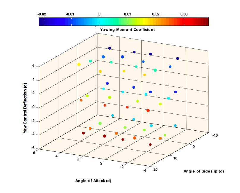
Example 10.
An excerpt from a sample aerodynamics model giving an example of a 3D
ungriddedTableDef element, encoding the data shown in Figure 3.
In this example, the dependent coordinates all vary in each dimension.
     <!--===================================-->
     <!--  Three-D Table Definition Example -->
     <!--===================================-->

     <ungriddedTableDef name="yawMomentCoefficientTable1" units="nd" utID="yawMomentCoefficientTable1">
                <!--  alpha,     beta,      delta:     yawMomentCoeff -->
       <dataPoint> -1.8330592 -5.3490387 -4.7258599 -0.00350641</dataPoint>
       <dataPoint> -1.9302179 -4.9698462 0.2798654  -0.0120538</dataPoint>
       <dataPoint> -2.1213095 -5.0383145 5.2146443  -0.0207089</dataPoint>
       <dataPoint> 0.2522004  -4.9587161 -5.2312860 -0.000882368</dataPoint>
       <dataPoint> 0.3368831  -5.0797159 -0.3370540 -0.0111846</dataPoint>
       <dataPoint> 0.2987289  -4.9691198 5.2868938  -0.0208758</dataPoint>
       <dataPoint> 1.8858257  -5.2077654 -4.7313074 -0.00219842</dataPoint>
       <dataPoint> 1.8031083  -4.7072954 0.0541231  -0.0111726</dataPoint>
       <dataPoint> 1.7773659  -5.0317988 5.1507477  -0.0208074</dataPoint>
       <dataPoint> 3.8104785  -5.2982162 -4.7152852 -0.00225906</dataPoint>
       <dataPoint> 4.2631596  -5.1695257 -0.1343410 -0.0116563</dataPoint>
       <dataPoint> 4.0470946  -5.2541017 5.0686926  -0.0215506</dataPoint>
       <dataPoint> -1.8882611 0.2422452  -5.1959304 0.0113462</dataPoint>
       <dataPoint> -2.1796091 0.0542085  0.2454711  -0.000253915</dataPoint>
       <dataPoint> -2.2699103 -0.3146657 4.8638859  -0.00875431</dataPoint>
       <dataPoint> 0.0148579  0.1095599  -4.9639500 0.0105144</dataPoint>
       <dataPoint> -0.1214591 -0.0047960 0.2788827  -0.000487753</dataPoint>
       <dataPoint> 0.0610233  0.2029588  5.0831767  -0.00816086</dataPoint>
       <dataPoint> 1.7593356  -0.0149007 -5.0494446 0.0106762</dataPoint>
       <dataPoint> 1.9717048  -0.0870861 0.0763833  -0.000332616</dataPoint>
       <dataPoint> 2.0228263  -0.2962294 5.1777078  -0.0093807</dataPoint>
       <dataPoint> 4.0567507  -0.2948622 -5.1002243 0.010196</dataPoint>
       <dataPoint> 3.6534822  0.2163747  0.1369900  0.000312733</dataPoint>
       <dataPoint> 3.6848003  0.0884533  4.8214805  -0.00809437</dataPoint>
       <dataPoint> -2.3347682 5.2288720  -4.7193014 0.02453</dataPoint>
       <dataPoint> -2.3060350 4.9652745  0.2324610  0.0133447</dataPoint>
       <dataPoint> -1.8675176 5.0754646  5.1169942  0.00556052</dataPoint>
       <dataPoint> 0.0004379  5.1220145  -5.2734993 0.0250468</dataPoint>
       <dataPoint> -0.1977035 4.7462188  0.0664495  0.0124083</dataPoint>
       <dataPoint> -0.1467742 5.0470092  5.1806131  0.00475277</dataPoint>
       <dataPoint> 1.6599338  4.9352809  -5.1210532 0.0242646</dataPoint>
       <dataPoint> 2.2719825  4.8865093  0.0315210  0.0125658</dataPoint>
       <dataPoint> 2.0406858  5.3253471  5.2880688  0.00491779</dataPoint>
       <dataPoint> 4.0179983  5.0826426  -4.9597629 0.0243518</dataPoint>
       <dataPoint> 4.2863811  4.8806558  -0.2877697 0.0128886</dataPoint>
       <dataPoint> 3.9289361  5.2246849  4.9758705  0.00471241</dataPoint>
       <dataPoint> -2.2809763 9.9844584  -4.8800790 0.0386951</dataPoint>
       <dataPoint> -2.0733070 9.9204337  0.0241722  0.027546</dataPoint>
       <dataPoint> -1.7624546 9.9153493  5.1985794  0.0188357</dataPoint>
       <dataPoint> 0.2279962  9.8962508  -4.7811258 0.0375762</dataPoint>
       <dataPoint> -0.2800363 10.3004593 0.1413907  0.028144</dataPoint>
       <dataPoint> 0.0828562  9.9008011  5.2962722  0.0179398</dataPoint>
       <dataPoint> 1.8262230  10.0939436 -4.6710211 0.037712</dataPoint>
       <dataPoint> 1.7762123  10.1556398 -0.1307093 0.0278079</dataPoint>
       <dataPoint> 2.2258599  9.8009720  4.6721747  0.018244</dataPoint>
       <dataPoint> 3.7892651  9.8017197  -4.8026383 0.0368199</dataPoint>
       <dataPoint> 4.0150716  9.6815531  -0.0630955 0.0252014</dataPoint>
       <dataPoint> 4.1677953  9.8754433  5.1776223  0.0164312</dataPoint>
     </ungriddedTableDef>